RSP Feedback Exercises
The following exercises are designed as a usability and functionality test of the Portal Aspect of the Rubin Science Platform (RSP; data.lsst.cloud). The goal is to understand how users interact with the Portal and identify areas that may require improvement. These exercises were also designed to serve also as challenged-based learning opportunities, complementary to the Documentation and tutorials.
Who can participate? Anyone with an RSP account at data.lsst.cloud.
How to participate? There are six exercises to choose from, two each at the beginner, intermediate, and experienced levels. Choose an exercise (use the table of contents at upper right), work through it, then complete the Feedback form. The entire process should not take more than 25 minutes per exercise, and might be much faster depending on RSP experience.
Resources. First, try the exercise on its own, then use any of these resources which are relevant: the DP0.2 documentation, DP0.2 schema browser, and DP0.2 Portal tutorials; the DP0.3 documentation, DP0.3 schema browser, and DP0.3 Portal tutorials; and the Portal (Firefly) Help pages (image display).
Answer key. In some cases, there are multiple ways to achieve a task in the RSP. Find at least one demonstration per exercise in the Portal Usability Test Answer Key
Feedback form
Thank you for completing the form, your feedback is essential and will be used by the Rubin Community Science Team (CST) to design processes to scientifically validate the RSP and enhance user experience.
The same form is used for all exercises.
Each exercise should take no more than 20 minutes; if it is taking longer, go to the feedback form and note that it couldn’t be finished in the time.
The feedback form is not anonymous and collects email addresses, so that CST members may follow up in some cases.
Link to this form: https://forms.gle/PdqNgW8ErV277tih9.
Exercise 1 (beginner)
Navigate in a web browser to data.lsst.cloud and log in to the Portal Aspect.
Select the “DP0.2 Catalogs” tab. This selection will default you to the “dp02_dc2_catalogs.Object” table.
Retrieve the g_psfFlux, g_calibFlux, and the g_extendedness columns
from the DP0.2 Object catalog for objects within 15 arcminutes of the galaxy cluster
at Right Ascension 55.75 degrees and Declination -32.27 degrees.
Plot the psfFlux vs. the calibFlux flux columns.
In the results table, impose a constraint to only plot objects with extendedness
equal to 1.
Change the plot symbols to open circles.
Reminder: If this task takes more than 20 minutes, please mark it as “could not be completed” in the feedback form and indicate how far you got.
Exercise 2 (beginner)
Create a g-r color vs. i magnitude diagram using the calibFlux columns in the DP0.2 Object catalog,
for all objects within 120 arcseconds of Right Ascension 60 degrees and Declination -35 degrees.
Zoom in on the clump of points with color values approximately in the range of -4 < g-r < 4.
Save the plot as a PNG file to your local computer. Hint: After retrieving the {band}_calibFlux columns,
use the expression (-2.5*log10({band}_calibFlux) + 31.4) to convert the fluxes in nanoJankys to magnitudes in the AB system.
Reminder: If this task takes more than 20 minutes, please mark it as “could not be completed” in the feedback form and indicate how far you got.
Exercise 3 (intermediate)
Retrieve the four DP0.2 processed visit images (PVI), also known as “calexp” images, obtained with LSST band i,
before the date of MJD 59840, whose boundaries contain the point with Right Ascension 55.75 degrees
and Declination -32.27 degrees. In the results view, choose the option to display the images in a grid.
Use the “Image center drop down” tool to center the first displayed image on the search coordinates.
Use the “Image alignment drop down” tool to align and lock all displayed images by the World Coordinate System (WCS)
and zoom-in 3 times.
Reminder: If this task takes more than 20 minutes, please mark it as “could not be completed” in the feedback form and indicate how far you got.
Exercise 4 (intermediate)
Use the ADQL interface to obtain, from the DP0.2 DiaSource table, an r-band light curve for the Type Ia supernova
which has a diaObjectId of 1250953961339360185. Retrieve the r-band fluxes and their errors derived from
a linear least-squares fit of a PSF model, and the effective mid-exposure time, for all diaSources associated
with this diaObjectId. Plot the light curve as the flux as a function of time, with error bars associated with
each flux point. Change the plot style to use connected points, the point style to be red circles, and then sort the
results by midPointTai.
Update the plot axes labels to be “PSF Difference-Image Flux” and “MJD of the Exposure Midpoint”.
Save the plot as a PNG file to your local computer.
Hint: In the ADQL query, the filter name will need to be
formatted as a string (e.g., 'r').
Reminder: If this task takes more than 20 minutes, please mark it as “could not be completed” in the feedback form and indicate how far you got.
Exercise 5 (experienced)
The following figure, which corresponds to Figure 15 from the
The LSST DESC DC2 Simulated Sky Survey paper,
has three panels: the grid of tracts in the DC2 simulation area on the left, the image of tract 3828 on the center,
and a zoom-in image approximately centered near a particularly bright elongated galaxy on the right.
The galaxy is located at Right Ascension = 3h46m56.21s and Declination = -36d05m27.7s (EQ_J2000).
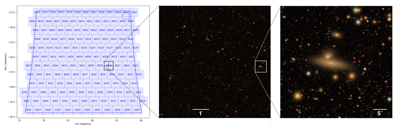
Figure 15 from the “The LSST DESC DC2 Simulated Sky Survey” paper.
Use the Portal Aspect of the RSP to reproduce the following figure, which shows an image of the same galaxy
in the r band, including:
The compass with cardinal points (N-E compass)
The footprint of the Hubble Space Telescope Wide Field Camera 3 - Infrared channel (WFC3/IR)
The extraction of a light profile of the galaxy. Save the light profile as a CSV file.
Hint: Use a color stretch “Linear: Stretch -1 Sigma to 30 Sigma” to resemble the figure below.
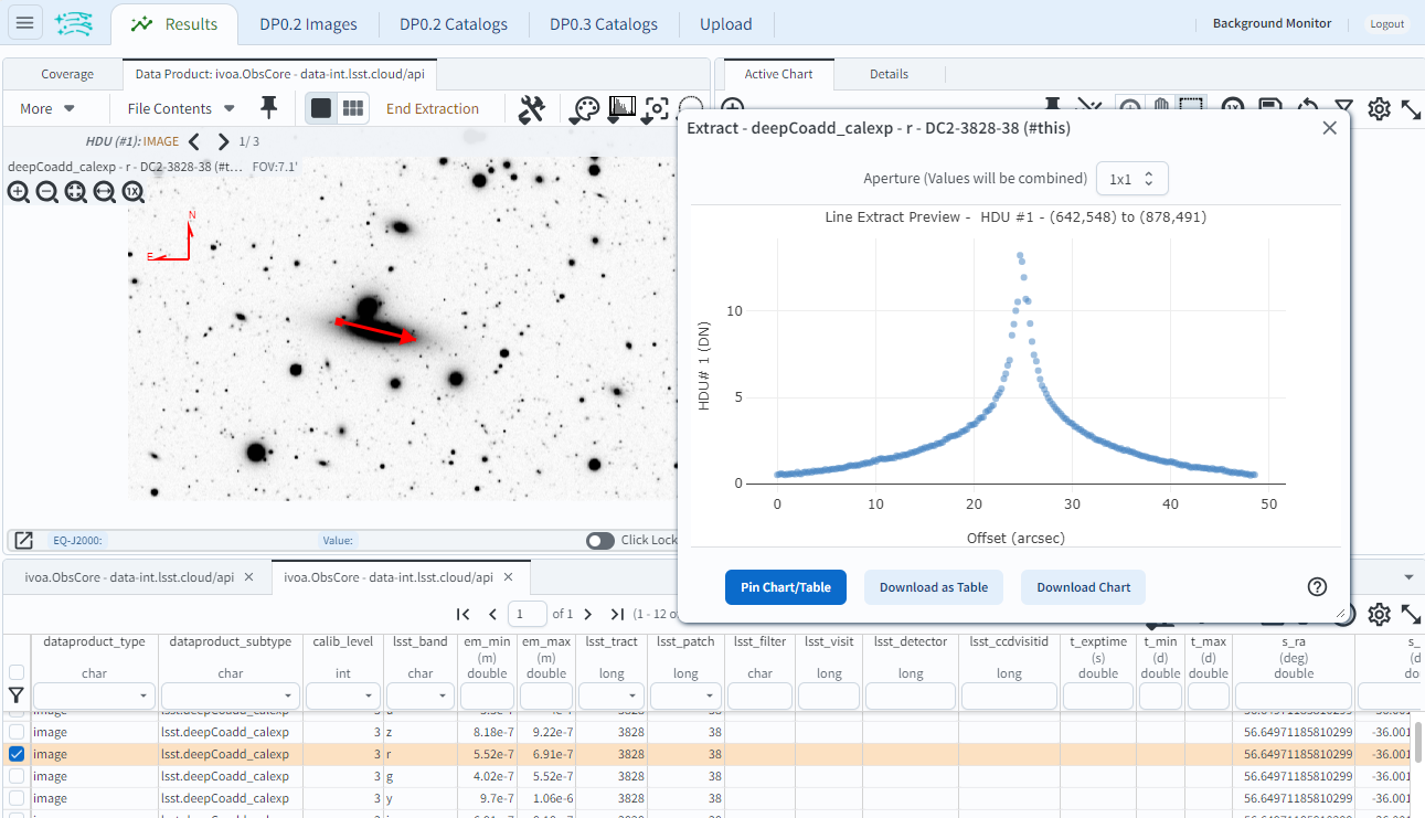
Screenshot of a DC2 galaxy from the Portal Aspect of the RSP.
Reminder: If this task takes more than 20 minutes, please mark it as “could not be completed” in the feedback form and indicate how far you got.
Exercise 6 (experienced)
Query the DP0.2 Object catalog for the galaxy cluster around Right Ascension 3h43m00.00s and Declination -32d16m19.00s
to visualize the region where the cluster is and plot the “red sequence” in a color-magnitude diagram
(for example, r-i vs i), as illustrated in the image below.
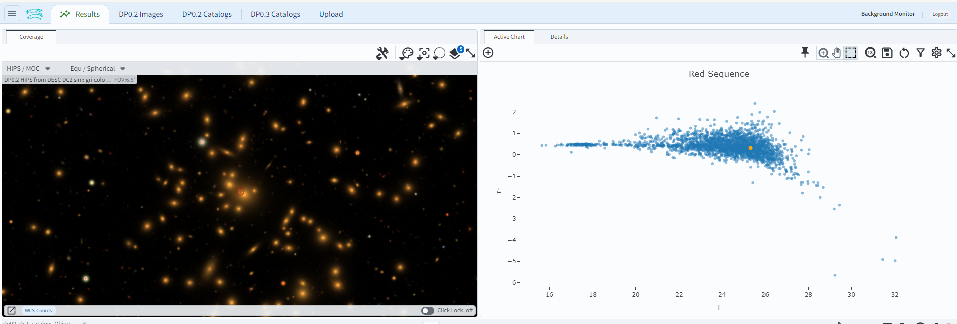
Screenshot of a DC2 galaxy from the Portal Aspect of the RSP.
Then, select the points in the red sequence to highlight the cluster members in the image, as shown in the image below.
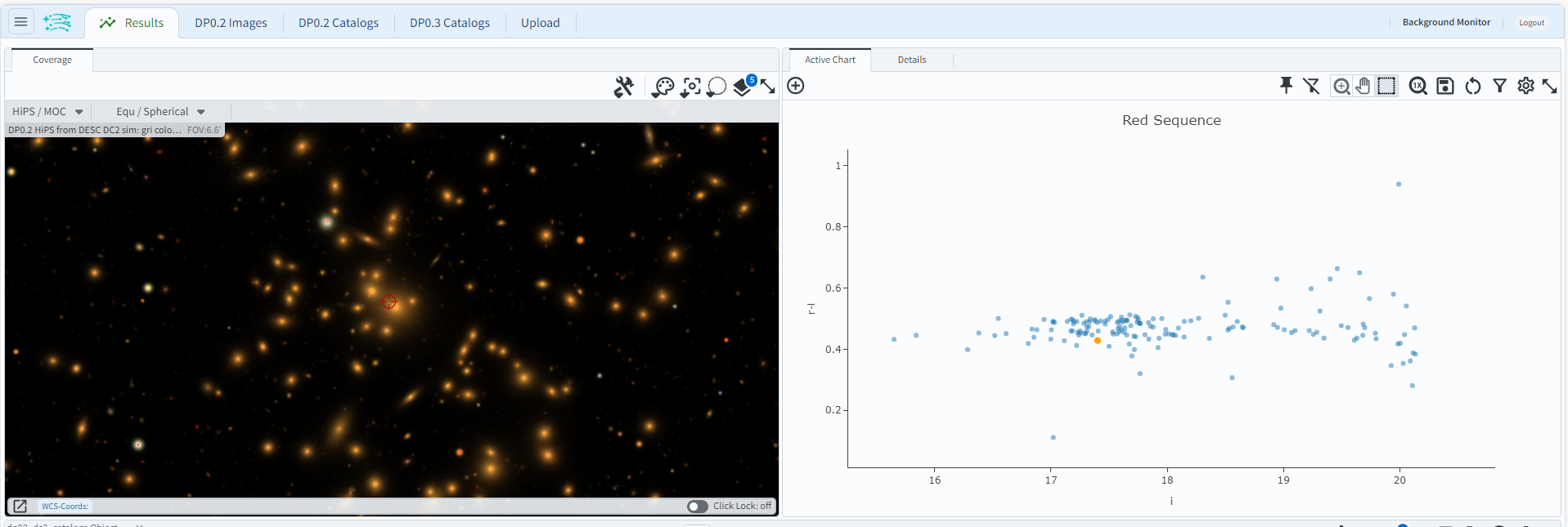
Hint 1: use a search radius of 200 arcseconds.
Hint 2: you can use the scisql_nanojanskyToAbMag SQL function to convert
fluxes to magnitudes (filter out negative fluxes before using the function).
Definition: The red sequence in galaxy clusters refers to a tight correlation observed in color-magnitude diagrams, where many of the galaxies in a cluster show a similar red color and brightness, indicating they are older, more evolved galaxies with less star formation.
Reminder: If this task takes more than 20 minutes, please mark it as “could not be completed” in the feedback form and indicate how far you got.